Advanced Tutorial

Welcome to the ECAgent Advanced Tutorial. In this tutorial we will be covering the following topics:

• Tags

• Class Components

• Environments

• Basic Data Collection

Before we get started, it is highly recommended that you first do the Introductory Tutorial before tackling this work. Note: This tutorial also assumes you are using ECAgent >= 0.5.5.

For this tutorial, we’ve decided to implement a simple predator-prey model as described by Tatara et al. (2006). They used this model to demonstrate the capabilities of Repast Simphony so, given our goal to do the same for ECAgent, it seems appropriate.

In this model, there are three types of entities (agents): Sheep, Wolves and Grass. The Sheep eat the Grass, the Wolves eat the Sheep and Grass regrows after a random amount of time. The model is intended to show very basic population dynamics namely, the carrying capacity of an ecosystem with predation.

Both the sheep and wolves expend energy every time they move. They gain energy by consuming the appropriate resource. If either a sheep or wolf gains enough energy, it gives birth. If they run out of energy, the die. The rate at which sheep and wolves consume energy and reproduce should be user-configurable parameters.

Components

With all that in mind, we’ll first create our model’s Components:

import numpy
import ECAgent.Core as Core

# Energy Component
class EnergyComponent(Core.Component):
    def __init__(self, agent, model, energy: float):
        super().__init__(agent, model)
        self.energy = energy  # The creatures remaining energy

# Species Class Component
class SpeciesComponent(Core.Component):
    def __init__(self, agent, model, prefix, gain, reproduce_rate):
        super().__init__(agent, model)
        # id prefix
        self.prefix = prefix
        # Energy gain for consuming food item
        self.gain = gain
        # Reproduction rate of Species
        self.reproduce_rate = reproduce_rate
        # Used to ensure agents have unique id per species
        self.counter = 0

The EnergyComponent is self-explanatory, it stores a float which denotes the amount of energy an agent has remaining.

The SpeciesComponent is slightly more complex. It contains several attributes, namely: prefix, gain, reproduce_rate and counter. What is interesting about these properties though is that, unlike energy in the EnergyComponent, none of the SpeciesComponent attributes are unique to any one agent. As the name suggests, they are unique to the species of the Agent (Sheep or Wolf which we are about to create). It would be inefficient , and tedious, to add a SpeciesComponent to every agent and ensure their values synced-up per agent species. We will alleviate this issue by using class components but let’s first create our Agent classes.

Agents

As noted earlier, the predator-prey model has 3 entity-types (Sheep, Wolves and Grass). Given the simplicity of the Grass entity, we are not going to create a specific class for it and instead will add it to our environment directly later.

To create our Sheep and Wolf agents, we do the following:

# Setup agent tags
import ECAgent.Tags as Tags

# Add Sheep Tag
Tags.add_tag('SHEEP')
# Add Wolf Tag
Tags.add_tag('WOLF')

# Sheep Agent
class Sheep(Core.Agent):
    def __init__(self, model, energy: float = None):
        # Get SpeciesComponent
        sp_comp = Sheep[SpeciesComponent]
        # Create agent id
        agent_id = f'{sp_comp.prefix}{sp_comp.counter}'
        super().__init__(agent_id, model, tag=Tags.SHEEP)
        # Add Energy Component
        self.add_component(
            EnergyComponent(
                self, model, energy if energy is not None
                else model.random.random() * 2 * sp_comp.gain
            )
        )
        sp_comp.counter += 1

# Wolf Agent
class Wolf(Core.Agent):
    def __init__(self, model, energy: float = None):
        # Get SpeciesComponent
        wlf_comp = Wolf[SpeciesComponent]
        # Create agent id
        agent_id = f'{wlf_comp.prefix}{wlf_comp.counter}'
        super().__init__(agent_id, model, tag=Tags.WOLF)
        # Add Energy Component
        self.add_component(
            EnergyComponent(
                self, model, energy if energy is not None
                else model.random.random() * 2 * wlf_comp.gain
            )
        )
        wlf_comp.counter += 1

This may look like a lot but, it’s only slightly more complex than what we did in the introductory tutorial. Before we get too deep into explaining the design of our agents, let’s first talk about Tags.

Tags

When designing Agent-Based Models (ABM), you may find yourself designing agents that are structurally similar (i.e. have similar components). This can make it difficult to customize their behaviour if you don’t have a method for uniquely identifying them. That’s were Tags come in. Found in the ECAgent.Tags submodule, we can make use of a TagLibrary to create a list of unique tags to identify our agents with.

Above, we used the global TagLibrary and simply created two new tags with the add_tag method. We can get a list of tags available in the TagLibrary by doing the following:

Tags.itemize()

[('NONE', 0), ('SHEEP', 1), ('WOLF', 2)]

As you can see, SHEEP and WOLF tags have been created for us. You will also notice a NONE tag which always exists in any TagLibrary and has a value of 0.

With this, we can now label our Sheep and Wolf agents which we do when we call their base class’ constructor using:

super().__init__(agent_id, model, tag=Tags.TAG_VALUE)

where TAG_VALUE is either SHEEP or WOLF.

The rest of the Sheep and Wolf classes are pretty standard where we ensure each agent has a unique id, add an EnergyComponent to them and give them a random energy value based on the species’ gain. If we don’t specify an energy value when initializing the agent.

You will also notice that we seem to be making use of a SpeciesComponent but never explicitly added it to our agents, that is where Class Components come in.

Class Components

As mentioned before, it makes no sense to instantiate some components more than once. The SpeciesComponent is a good example of this because each agent of a particular species doesn’t need their own SpeciesComponent, they can all simply use the same one by virtue of being the same species.

With that in mind, how to actually achieve this? Well, in ECAgent we do this by binding or attaching components to an Agent’s class. In other words, we create a class component, or a component that is the same component for all agents of the same type/class.

We do this by doing the following:

# Add Species Component to Sheep Class
Sheep.add_class_component(SpeciesComponent(Sheep, model))

Note: that we won’t run this code right now since we don’t have a model object to pass to the component just yet.

The takeaway from the example though, is that we can add a component to a class, and we do that by calling the add_class_component method. The ‘agent’ this component belongs to is then the Agent class itself, not any instanced object as is the case with regular components.

To access a class component, you can use get_class_component(ComponentType) or the [ComponentType] shorthand we used when creating our agent classes (which is the same way you can access components on instantiated agent objects).

Environments

ABM environments are not clearly defined. They can be void of characteristics or incredibly detailed recreations of real-world locations. Discretized multi-dimensional lattices or graph structures are common. In this tutorial, we will be making use of such a structure called a GridWorld.

Simply put, a GridWorld is a two-dimensional grid-like environment where each grid cell represents a distinct location with unique x and y-coords. For example, a 3x3 GridWorld will look as follows:

__	__	__
(0, 2)	(1, 2)	(2, 2)
(0, 1)	(1, 1)	(2, 1)
(0, 0)	(1, 0)	(2, 0)

where (x,y) are the x and y-coordinates of the environment.

To make use of a GridWorld environment, we must first import the submodule:

from ECAgent.Environments import GridWorld, PositionComponent, discrete_grid_pos_to_id

The ECAgent.Environments submodule contains several types of environments that you can make use of including a continuous environment called a SpaceWorld and the GridWorld we will be using in this tutorial.

When an agent is added to a GridWorld (or any spatial environment for that matter), it is automatically given a component called a PositionComponent. You do not need to create this component yourself, but you can access it by calling get_component(PositionComponent) on any agent that has been added to the GridWorld environment.

For clarity, the PositionComponent is a simple class that stores an agent’s x, y and z-coordinates:

# Taken from ECAgent.Environments
class PositionComponent(Component):
    def __init__(self, agent, model, x = 0.0, y = 0.0, z = 0.0):
        super().__init__(agent, model)
        self.x = x
        self.y = y
        self.z = z

We will not be making use of the z attribute since we will only be working in two dimensions.

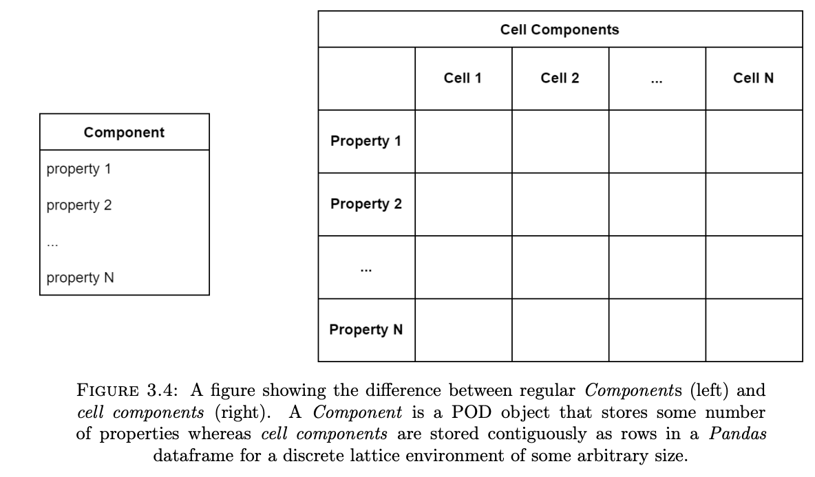
The last aspect of the GridWorld we need to talk about is cell components. Recall that our predator-prey model consists of Grass entities that we have yet to create. Well it turns out that for each cell in our GridWorld, we need a Grass entity. Now consider a simple 10x10 GridWorld, we would need 100 Grass entities. If we wanted to add a component to the Grass entities, we would need to instantiate 100 of these components every time. Simply put, this is incredibly memory inefficient and will increase our model’s execution time significantly (more so for much larger GridWorld environments).

To combat this, we can make use of cell components which, under the hood, store components in a memory efficient manner. The catch is that these attributes need to be simple primitives (int, float, etc.). The following figure demonstrates the distinction between a standard Component and a cell component:

To create a cell component you can simply use:

environment.add_cell_component('name', data)

where environment is a GridWorld, 'name' is the cell component’s name and data is the initial values of said attribute for each cell in the GridWorld. You can use Generators to write custom initialization functions for each cell but a simpler solution is to just supply the data directly using a list or np.ndarray:

# Assumes a 3x3 GridWorld
data = [0, 1, 2, 3, 4, 5, 6, 7, 8]
environment.add_cell_component('coins', data)

The above code will create a 'coins' attribute which when viewed directly will just like a regular array:

[0, 1, 2, 3, 4, 5, 6, 7, 8]

However, when viewed from the perspective of a GridWorld will look like:

__	coins	__
6	7	8
3	4	5
0	1	2

Systems

Now that we have a basic understanding of our environment, we can create our systems. For this work, we will be creating four:

• MovementSystem: Responsible for moving the Sheep and Wolf agents within the environment.

• ResourceConsumptionSystem: The system responsible for managing the consumption of new resources. This includes sheep eating grass, wolves eating sheep and grass regrowing.

• DeathSystem: The system responsible for removing sheep and wolves with no energy remaining.

• BirthSystem: The system responsible for stochastically adding new sheep and wolves to the simulation.

MovementSystem

Let’s first create our MovementSystem as follows:

class MovementSystem(Core.System):
    def __init__(self, id: str, model):
        super().__init__(id, model)

    def execute(self):
        # For each agent in the environment
        for agent in self.model.environment:
            # Move within Moore Neighbourhood [-1, 1]
            x_offset = round(2 * self.model.random.random() - 1)
            y_offset = round(2 * self.model.random.random() - 1)
            self.model.environment.move(agent, x_offset, y_offset)

            # Spend Energy
            agent[EnergyComponent].energy -= 1

As usual, we override the execute() method. We then iterate over every agent using a for loop. For each agent, we randomly assign it a new position within its Moore Neighbourhood. We use model.random to ensure that the model’s pseudorandom number generator is used. Note that we make use of the built-in environment.move() function because it automatically handles cases where agents move out of bounds. We could do the movement ourselves by manually accessing the PositionComponent of each agent as follows:

# Note this doesn't do any bound checking
agent[PositionComponent].x += x_offset
agent[PositionComponent].y += y_offset

ResourceConsumptionSystem

The next System to create is the ResourceConsumptionSystem which is the most complex part of the model given that it strays from traditional OOP design principles. It is implemented as follows:

class ResourceConsumptionSystem(Core.System):
    def __init__(self, id: str, model, regrow_time: int):
        super().__init__(id, model)
        self.regrow_time = regrow_time

        def resource_generator(pos, cells):
            return 1 if model.random.random() < 0.5 else 0

        # Generate the initial resources
        model.environment.add_cell_component('resources',
                                           resource_generator)

        def countdown_generator(pos, cells):
            return int(model.random.random() * regrow_time)

        # Generate the initial resources
        model.environment.add_cell_component('countdown', countdown_generator)

    def execute(self):
        # Get resources data
        cells = self.model.environment.cells
        resource_cells = cells['resources'].to_numpy()
        countdown_cells = cells['countdown'].to_numpy()
        eaten_sheep = []
        targets_at_pos = {}
        environment = self.model.environment
        # Process Sheep and Wolves first

        for agent in environment:
            posID = discrete_grid_pos_to_id(agent[PositionComponent].x, agent[PositionComponent].y,
                                            self.model.environment.width)

            # Is wolf or is sheep
            if agent.tag == Tags.WOLF:
                # Get all agents at position
                if posID not in targets_at_pos:
                    targets_at_pos[posID] = environment.get_agents_at(
                        agent[PositionComponent].x, agent[PositionComponent].y)

                for target in targets_at_pos[posID]:
                    # If sheep
                    if target.tag == Tags.SHEEP and target.id not in eaten_sheep:
                        # Mark Sheep for death
                        eaten_sheep.append(target.id)
                        # Wolf gets energy for eating Sheep
                        agent[EnergyComponent].energy += Wolf[SpeciesComponent].gain
                        break

            elif agent.id not in eaten_sheep:
                # Check is grass is Alive
                if resource_cells[posID] > 0:
                    # Sheep consumes Grass and gains Energy
                    agent[EnergyComponent].energy += Sheep[SpeciesComponent].gain
                    resource_cells[posID] = 0

        # Remove eaten sheep
        for sheep in eaten_sheep:
            environment.remove_agent(sheep)

        # Regrow Grass
        countdown_cells[resource_cells < 1] -= 1
        mask = countdown_cells < 1
        resource_cells[mask] = 1
        countdown_cells = numpy.where(mask, numpy.asarray(
        [
            int(self.model.random.random() * self.regrow_time)
            for _ in range(len(countdown_cells))
        ]), countdown_cells)

        # Update grass levels and countdowns in environment
        self.model.environment.cells.update({
            'resources': resource_cells,
            'countdown': countdown_cells
        })

The above code is quite lengthy so here a short description of the interesting bits. First, you’ll notice that this system has a regrow_rate input parameter. At initialization, we’ll provide a value which specifies the maximum number of iterations a grass entity will be inactive for.

We then add two cell components to the model using environment.add_cell_component. We pass the name of the cell components (resources and countdown respectively) and two generator functions which describe the initial value of each cell.

Generator function have a particular form:

def generator_name(pos, cells):
    do some stuff...
    return value_of_cell

where pos is a tuple with the coordinates of the cell and cells is a DataFrame that stores all the cell component data. Luckily our generators are quite simple with resource_generator randomly turning on about 50% of the grass (resource) patches. On the other hand, countdown_generator assigns a random value to the countdown attribute which describes how many iterations it will take for a dead grass cell to regrow.

In the execute() method, we loop over every agent and determine its posID. Given that the cell components are stored contiguously (i.e. In a 1D array), we need to convert the agent’s position from a 2D value, into a 1D value. We do this using the discrete_grid_pos_to_id() method included with ECAgent.Environments and store it as the posID. If the agent is a Wolf (i.e. agent.tag == Tags.WOLF), we get a list of all agents at its current position using the environment.get_agents_at() method and loop over them. If any one of them is a Sheep, the Wolf consumes it and gains energy equal to the value of Wolf[SpeciedComponent].gain (which you’ll recall is a class component that we created earlier). In this implementation, a Wolf will only eat one Sheep at a time.

If the agent is a Sheep, it will look to see if its current cell has any resources (i.e. the grass cell at position posID has a resource value of 1.0). If the cell has resources, it consumes them and gains energy equal to Sheep.gain. The resources at that current cell are then set to 0.0.

After both agent types have eaten, all dead Sheep are removed from the environment using environment.remove_agent(). The cells are then updated using Numpy masks and code vectorization. This code is can be hard to understand if you are not familiar with Numpy but what is happening is that the countdown cell component for all cells who currently have no resources (i.e. a resource component value of 0.0) is decremented by 1.0. We then check to see if any of these resource-less cells have reached a countdown value of 0.0 and if so, they are given a new random countdown value ∈ [0, regrow_time] and have their resource component set to 1.0. Because of Numpy’s code vectorization, these operations are applied to all cells simultaneously which is much faster than traditional OOP methods which typically evaluate each cell independently. Lastly, the new resources and countdown values are committed to the environment using environment.cells.update.

DeathSystem

The DeathSystem is self-explanatory. It is responsible for removing agents from the environment when their energy is depleted. It is implemented as follows:

class DeathSystem(Core.System):
    def __init__(self, id, model):
        super().__init__(id, model)

    def execute(self):
        toRem = []
        for agent in self.model.environment:
            if agent[EnergyComponent].energy <= 0:
                toRem.append(agent.id)

        for a in toRem:
            self.model.environment.remove_agent(a)

In the above code snippet, we loop over all agents and if their energy (which we get from by accessing the EnergyComponent) is less than or equal to 0, we remove the agent using environment.remove_agent(). The method takes the agent’s id as input.

BirthSystem

Similarly, the BirthSystem is just responsible for stochastically adding new Sheep and Wolf agents to the environment. It is implemented as follows:

class BirthSystem(Core.System):
    def __init__(self, id, model):
        super().__init__(id, model)

    def execute(self):
        for agent in self.model.environment.get_agents():
            new_agent = None
            if agent.tag == Tags.WOLF and self.model.random.random() < Wolf[SpeciesComponent].reproduce_rate:
            # Birth Wolf
                agent[EnergyComponent].energy /= 2.0
                new_agent = Wolf(self.model,
                         energy=agent[EnergyComponent].energy
                    )

            elif self.model.random.random() < Sheep[SpeciesComponent].reproduce_rate:
            # Birth Sheep
                agent[EnergyComponent].energy /= 2.0
                new_agent = Sheep(self.model,
                        energy=agent[EnergyComponent].energy
                )

            # Add agent to environment (at its parent's location)
            if new_agent is not None:
                self.model.environment.add_agent(
                    new_agent, *agent[PositionComponent].xy()
                )

In the above code, we loop over all agents and check to see what type of agent they are by looking at the agent’s tag Both wolves and sheep reproduce in the same way, a random number ∈ [0, 1] is generated and if it is less than the agent type’s reproduce_rate, a new agent (of the same type) is spawned. Half the energy of the parent is given to the child agent. We add new agents to the environment using environment.add_agent. Lastly, the position of the child agent is set to that of the parent’s position.

Data Collection

Given that we are interested in monitoring both the Sheep and Wolf populations. It is probably worth developing a mechanism to record these values. We do that by making use of the Collector class as follows.

import ECAgent.Collectors as Collectors

class DataCollector(Collectors.Collector):
    def __init__(self, id: str, model):
        super().__init__(id, model)
        self.records = {'sheep': [], 'wolves': []}

    def collect(self):
    # Count Sheep
        self.records['sheep'].append(
            len(self.model.environment.get_agents(tag=Tags.SHEEP))
        )
    # Count Wolves
        self.records['wolves'].append(
            len(self.model.environment.get_agents(tag=Tags.WOLF))
        )

Collectors are a special type of System in ECAgent meant to record model or agent properties. Here we’ve just implemented a simple Collector called DataCollector. It inherits from Collector (not System) and overrides the collect() method (not the execute() method). During initialization, we setup a dictionary that will store the population of the sheep and wolves. When the collect() method is called, we count the number of sheep and wolves currently in the environment using environment.get_agents() and filtering each search by each species’ respective tag.

Putting it all together

With all of our Systems created, we can create our predator-prey model as follows:

class PredatorPreyModel(Core.Model):
    def __init__(self, size: int, init_sheep: int, init_wolf: int,
        regrow_rate: int, sheep_gain: float, wolf_gain: float,
        sheep_reproduce: float, wolf_reproduce: float, seed: int = None):
        super().__init__(seed=seed)

    # Create Grid World
        self.environment = GridWorld(self, size, size)

    # Add Systems
        self.systems.add_system(MovementSystem('move', self))
        self.systems.add_system(ResourceConsumptionSystem('food',
            self, regrow_rate))
        self.systems.add_system(BirthSystem('birth', self))
        self.systems.add_system(DeathSystem('death', self))
        self.systems.add_system(DataCollector('collector', self))

    # Add Class Components
        Wolf.add_class_component(
            SpeciesComponent(Wolf, self, 'w', wolf_gain,
                             wolf_reproduce)
        )
        Sheep.add_class_component(
            SpeciesComponent(Sheep, self, 's', sheep_gain,
                             sheep_reproduce)
        )

    # Create Agents at random locations
        for _ in range(init_sheep):
            self.environment.add_agent(
                Sheep(self),
                x_pos = self.random.randint(0, size - 1),
                y_pos = self.random.randint(0, size - 1)
            )

        for _ in range(init_wolf):
            self.environment.add_agent(
                Wolf(self),
                x_pos = self.random.randint(0, size - 1),
                y_pos = self.random.randint(0, size - 1)
            )

    # Method that will execute Model for t timesteps
    def run(self, t: int):
        self.execute(t)

Perusing the code, you’ll notice that upon initialization, the model accepts nine input parameters:

1. Size: The size of the GridWorld. This value dictates both the width and height of the grid world (i.e. The GridWorld is square).

2. Initial Sheep: The number of Sheep agents to initialize.

3. Initial Wolves: The number of Wolf agents to initialize.

4. Regrowth rate: The max number of iterations it will take for a grass cell to regrow.

5. Sheep Gain: The amount of energy a Sheep gains when it consumes a grass cell.

6. Wolf Gain: The amount of energy a Wolf gains when it consumes a Sheep.

7. Sheep Reproduction Rate: The rate at which Sheep agents spawn additional Sheep agents.

8. Wolf Reproduction Rate: The rate at which Wolf agents spawn additional Wolf agents.

9. Seed: The seed for the pseudo-random number generator.

These are the same parameters specified by Tatara et al. (2006) and are intended to be user configurable. The first thing we do is create the GridWorld that the agents will occupy. The Model class adds a basic (dimensionless) environment by default. By creating the GridWorld, we ensure that any agents added to the environment will automatically get a PositionComponent attached to them. We can also now create cell components which are not available in the basic Environment. The size of the GridWorld is set to be the value of the size parameter.

Each System is added using the systems.add_system() method and given a unique string id. We do not specify the priority, frequency, start or end properties in this case. This is because we want our Systems to execute every iteration, from iteration zero until the end of the simulation run. By not specifying a priority, the SystemManager treats the execution order as ’first-come first serve’ meaning that MovementSystem will always execute first and the DataCollector will always execute last. If this didn’t make sense to you, it may be worth reading up on how the execution order of Systems is determined here.

We then specify some other user configurable properties gain and reproduce for both the Sheep and Wolf agent types. We do this by creating a SpeciesComponent for each agent-type and add them as class components using add_class_component() Lastly, we create our agents (and add them to environment) using the environment.add_agent() method. Each agent’s position is randomly assigned to somewhere on the grid world.

Visualization and Validation

The last thing to do is visualize the results produced by our model. We can do this in a number of ways but the easiest is to just take the recorded population levels and plot as follows:

import matplotlib.pyplot as plt

# Input Parameters

ENV_SIZE = 50
INIT_SHEEP = 100
INIT_WOLF = 50
REGROW_RATE = 30
SHEEP_GAIN = 4
WOLF_GAIN = 25
SHEEP_REPRODUCTION = 0.04
WOLF_REPRODUCTION = 0.06

# Change this to change length of simulation
ITERATIONS = 1000
SEED = 345968  # For pseudo-random number generator

model = PredatorPreyModel(
        ENV_SIZE,
        INIT_SHEEP,
        INIT_WOLF,
        REGROW_RATE,
        SHEEP_GAIN,
        WOLF_GAIN,
        SHEEP_REPRODUCTION,
        WOLF_REPRODUCTION,
        SEED)

# Execute model (May take some time based on input params used)
model.run(ITERATIONS)

# Get population levels from data collector
records = model.systems['collector'].records

# Create Matplotlib Plots
fig, ax = plt.subplots()
ax.set_title('Sheep and Wolf Populations in \nSimple Predator Prey Model')
ax.set_xlabel('Iterations')
ax.set_ylabel('Population')

iterations = numpy.arange(ITERATIONS)

for species in records:
    ax.plot(iterations, records[species], label=species)

ax.legend(loc='lower right')
ax.set_aspect('auto')
plt.show()

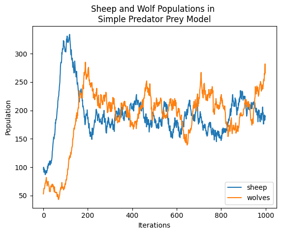
That’s it! When you run the code you should see a plot appear. You’ll know the model is working if you see the population levels oscillating between Sheep and Wolf carrying capacities.

We covered a lot in this tutorial, it may be worthwhile to reread some concepts you are unfamiliar with. If you are still lost, take a look the documentation or go over some other examples we have available (TODO).

For now, play around with the model’s input parameters and see what interesting phenomena emerge.